Homeomorphism Methods

A feasible set, in different coordinates

Let $K$ be the set of admissible decisions, and let $B$ be the unit ball: all coordinates with length at most one. In our 2D figures, $B$ is a filled disk. The point $z$ is a reference coordinate; $x$ is the actual decision. A homeomorphism $\Phi$ pairs every $z$ in $B$ with exactly one $x$ in $K$, and its inverse $\Phi^{-1}$ takes $x$ back to $z$. Both directions are continuous: small changes remain small in either coordinate system. This does not mean that distances are preserved.

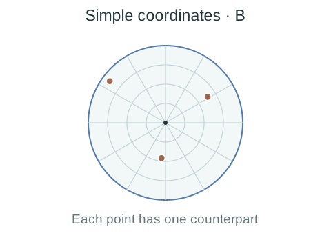
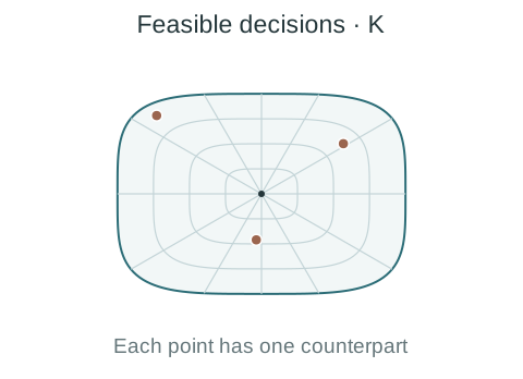
Why is this useful? If $\Phi(B)=K$, choosing a valid coordinate $z$ is enough to construct a feasible decision. We have moved constraint handling into the representation. The ball still imposes a constraint, but clipping a point to a ball is a simple calculation.

Invertibility adds something beyond an ordinary feasible decoder: we can also bring existing decisions and training data back into reference coordinates. The same map can therefore support several tasks. A homeomorphism preserves topology; it can still stretch distances and change the appearance of the region.

Constructing the map: follow a ray

For a compact convex set with nonempty interior, a gauge map gives a concrete construction. Choose an interior point $x_0$. From that point, every direction reaches the boundary at a well-defined distance. Use this distance to scale the corresponding radius of the ball.

Write $z=ru$, where $u$ is a unit direction and $0\le r\le1$. If $R(u)$ is the distance from $x_0$ to the boundary along $u$, the map is

A radius halfway to the ball boundary lands halfway along the corresponding target ray. A point on the sphere lands on the target boundary. The direction identifies the ray; $r$ identifies the relative position along it.

Earlier examples in learning-based control come from Tabas and Zhang. They use gauge maps to turn bounded neural-network outputs into state-dependent safe actions for reinforcement learning,^[1] and into feasible control sequences for model predictive control (MPC).^[2] Their reference domain is an $\ell_\infty$ unit ball—a box with each coordinate between −1 and 1—rather than the Euclidean ball illustrated here. The shared principle is to rescale rays from an interior point, so that simple reference coordinates represent admissible decisions.

What to notice: radius 0 maps to the center, and radius 1 maps to the boundary. Changing direction selects a different ray in both domains.

The explorer also shows a nonconvex star-shaped region. Its positive, continuous radial boundary still lets each ray serve as a coordinate. This construction illustrates why the idea can extend beyond convex sets; an arbitrary nonconvex region need not admit such a map.

Computing R is the practical step. Common linear, quadratic, and conic constraints provide structured boundary calculations; general convex constraints can use a one-dimensional boundary search. The original constraint description still determines the cost. The implementation contains these calculations.

Further detail: slides 10–12 ↗ and slide 50 ↗.

Learning: recover a usable prediction

The coordinate idea reaches learned predictions in two ways: ask the network to predict coordinates directly, or recover a decision after it has been predicted.

Construct the output in feasible coordinates. With an exact map onto the feasible set, a network can predict $z$, enforce $z\in B$, and return $\Phi(z)$. For input-dependent constraints, use the map for that input. Training through the decoder lets the model account for how its coordinates become decisions. A related feasible-output construction appears in RAYEN, an output layer that enforces supported convex constraints.^[3]

Recover a prediction after it is made. The predictor learns a decision; a separate invertible network learns the coordinate map. Coupling-based networks are one established choice, with approximation properties studied by Teshima et al.^[4] Homeomorphic Projection inverse-maps the prediction, recovers a feasible point in those coordinates, and maps it back.^[5]

Recovery starts from a center whose mapped decision is known to be feasible. Move the prediction’s reference coordinate toward that center. Bisection repeatedly tests a midpoint along this path: map it back, check the original constraints, and keep a feasible endpoint as the search narrows. Return the mapped feasible endpoint. This check matters because invertibility alone does not make the learned ball image equal to the true feasible set.

The recovered decision generally differs from the Euclidean nearest feasible point. A map that stretches some directions strongly can produce a larger correction. This motivates learning a map with small distortion: it helps preserve the quality of an already useful prediction. The paper relates the loss to prediction error, map approximation, distortion, and bisection accuracy.

Further detail: slides 32–34 ↗.

Optimization: improve the decision inside the ball

Now keep the objective explicit. We want to minimize $f(x)$ over $x\in K$. With an exact homeomorphism, this is equivalent to minimizing the composite objective $h(z)=f(\Phi(z))$ over $z\in B$. Every feasible decision has a coordinate, so the best objective value is preserved.

The potential saving is in constraint handling: replace an expensive projection onto $K$ with a cheap ball projection plus map evaluation and differentiation. Hom-PGD takes a gradient step on the transformed objective, projects onto $B$, and maps the iterate back.^[6] With step size $\eta$, the update is

$\Pi_B$ is projection onto the unit ball: keep a point if its length is at most one; otherwise divide it by its length. The gradient $\nabla h$ is taken with respect to the reference coordinate $z$, so it accounts for how the map changes the decision. The method avoids projection onto the original set $K$; feasibility of each decoded iterate relies on the map and numerical operations.

Changing coordinates can also change the objective landscape: convexity is not generally preserved by a nonlinear map. Under the paper’s regularity assumptions, Hom-PGD matches standard unaccelerated first-order convergence rates. Map distortion affects the constants and practical conditioning, and the choice of interior center can influence speed. The paper explains these effects in more detail.

Further detail: slides 9–15 ↗.

Sampling: learn the distribution in simple coordinates

Learning and optimization often aim to return one good decision. Sampling adds a different goal: producing a collection of feasible outputs with the right variation. A planner may need several plausible routes, or a scientific generator may need diverse candidates. The probability assigned to different regions matters.

Flow matching learns a velocity field that moves samples from a simple starting distribution toward the data distribution.^[7] Reflected Flow Matching develops this idea for bounded domains by handling their boundaries.^[8] Intuitively, reflection adjusts proposed motion at the boundary to keep samples inside.

Gauge Flow Matching brings these ingredients into reference coordinates.^[9] Map feasible training data back to the ball with $\Phi^{-1}$, then train a velocity field on that transformed distribution. At inference, start from a prior supported inside $B$, use reflected flow sampling within $B$, and map the generated coordinates into $K$.

Keeping the sampler in $B$ is part of the method. An unconstrained numerical flow can leave the ball; invertibility by itself does not prevent that. An exact feasible map can transfer ball-space feasibility to the output, while the learned flow determines how closely the resulting distribution matches the data.

Mapping points also moves probability mass

Uniform draws in the ball generally become nonuniform after mapping. A region that expands under $\Phi$ receives the same probability mass spread over more area. A compressed region receives denser mass.

Read the point clouds: each point keeps its probability weight. Where does the map spread that weight over more area?

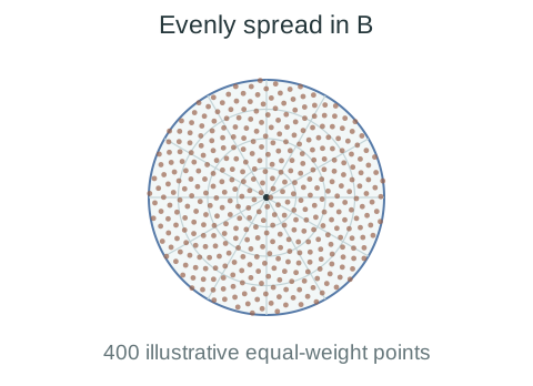
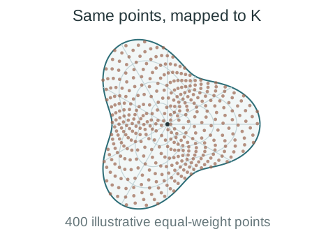
These clouds illustrate probability transport, rather than a trained GFM result. This is why GFM learns from inverse-mapped data, rather than assuming a uniform ball prior already represents the desired output law. The same probability-transport principle underlies normalizing flows: for a smooth invertible map, its local volume change determines the density change.^[10] Feasibility, distribution accuracy, and sampling cost remain separate questions.

Further detail: slides 49–51 ↗.

The map must fit the geometry

The shared framework is attractive when a useful map exists and is cheap to evaluate in both directions. Three features determine whether it is a good fit.

• Topology. A disk can deform into a filled nonconvex shape with the same topology. It cannot map homeomorphically onto an annulus with a hole or a disconnected set. Such domains require a different reference space, multiple charts, or another method.
• Dimension. Equality constraints can reduce the number of independent variables. Work in those reduced coordinates and reconstruct the dependent variables when a suitable parameterization exists. A full-dimensional ball cannot be treated as a homeomorphic representation of an arbitrary lower-dimensional feasible surface.
• Distortion and computation. Continuity and invertibility establish a correspondence; bi-Lipschitz control additionally limits stretching and compression. These properties matter for correction quality, optimization conditioning, and distribution error. They must be weighed against map construction, evaluation, and any constraint checks. Here, bi-Lipschitz means that both the map and its inverse have bounded stretching.

For convex bodies, a gauge map offers a direct route. For more general ball-homeomorphic sets, learning the map can be useful, but invertibility, domain coverage, and constraint satisfaction need distinct checks. Homeomorphism is a framework for organizing the problem, and the chosen construction supplies the operational details.

One change of coordinates, three uses

The common move is to represent feasible decisions through a simpler domain. What happens in that domain depends on the task: recover a prediction through checked coordinate search, optimize the transformed objective, or learn and sample a transformed distribution.

When evaluating a method, ask three questions: does the returned object satisfy the constraints, does it retain the quality or distribution we need, and what is the total cost? A useful coordinate system helps with all three, but each still needs its own evidence.

For the full development, see the slides and the papers below. Implementations are available for Homeomorphic Projection, Hom-PGD, and Gauge Flow Matching.

Papers and further reading

The references cover feasible-output layers, invertible maps, optimization, and probability transport, alongside the three methods featured in this post.

1. Tabas and Zhang. Computationally Efficient Safe Reinforcement Learning for Power Systems. ACC, 2022 (preprint, 2021).
2. Tabas and Zhang. Safe and Efficient Model Predictive Control Using Neural Networks: An Interior Point Approach. CDC, 2022.
3. Tordesillas et al. RAYEN: Imposition of Hard Convex Constraints on Neural Networks. arXiv:2307.08336, 2023; updated 2026.
4. Teshima et al. Coupling-based Invertible Neural Networks Are Universal Diffeomorphism Approximators. NeurIPS, 2020.
5. Liang, Chen, and Low. Homeomorphic Projection to Ensure Neural-Network Solution Feasibility for Constrained Optimization. JMLR, 2024. ICML 2023 version.
6. Liu, Liang, and Chen. Fast Projection-Free Approach (without Optimization Oracle) for Optimization over Compact Convex Set. NeurIPS, 2025.
7. Lipman et al. Flow Matching for Generative Modeling. ICLR, 2023.
8. Xie et al. Reflected Flow Matching. ICML, 2024.
9. Li, Liang, and Chen. Gauge Flow Matching: Efficient Constrained Generative Modeling over General Convex Set and Beyond. ICLR, 2026.
10. Papamakarios et al. Normalizing Flows for Probabilistic Modeling and Inference. JMLR, 2021.