Suppose a model helps divide a one-unit budget between two services. It predicts 0.51 units for each—close to a reference allocation of 0.5, but together they exceed the budget. How do we turn a useful prediction into a decision we can actually use?
That question connects resource allocation, robot planning, and molecular generation: a promising candidate must also obey the rules of its task. We will use one budget triangle to compare constraint mechanisms, then follow the same question into diffusion and flow sampling.
Accurate, yet impossible to use
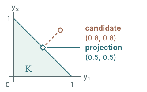
Even a small prediction error can break a hard constraint. To make the geometry visible, the figures below use a larger candidate: 0.8 units for each service, still against a budget of one. The shaded triangle contains every allocation we are allowed to return.
This is a different question from how much prediction error we can tolerate. Accuracy measures agreement with a reference output. Utility measures how well a decision serves the task, such as its cost or efficiency. Feasibility asks whether that decision obeys the rules. An accurate prediction can be infeasible, and a feasible decision can still be inefficient. These are three separate judgments.
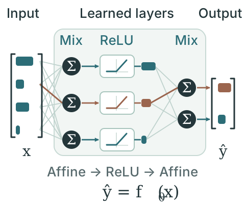
A neural network can learn to propose allocations from past solutions. The useful distinction is where feasibility comes from: the predictor, its output representation, or an operation applied to the candidate.
Draw the feasible set first
For our example, write the two allocations as and . They must be nonnegative, and their sum must not exceed one. The allowed outputs form a triangle:
The point sits outside this triangle. The points , , and lie inside or on its boundary. Whether those feasible points are good allocations is a separate question.
More generally, a feasible set can combine equalities, such as conservation laws, with inequalities, such as capacity limits. It may depend on an input: today's demand, the current robot state, or a requested output schema. We can write this as , where describes the instance. The important output is the final returned , after any decoding, completion, correction, or solve.
Calling a requirement hard says that it defines admissibility. It does not establish that a particular algorithm meets it. A formula may preserve feasibility exactly in mathematics; a numerical implementation works with finite precision. For a numerical solve, “feasible” usually means that the returned equality and inequality residuals meet explicit tolerances.
Our triangle is deliberately simple: a nonempty convex set with linear inequalities. Equality constraints can restrict outputs to a surface; nonconvex constraints can create holes or disconnected regions; discrete constraints can admit only isolated choices. A construction that works for the triangle does not automatically extend to those geometries. Drawing the set is the first step toward seeing which tools are available.
Can we just add a penalty?
A familiar approach adds a violation term to the training objective: task loss plus a weighted constraint penalty. This can use valuable knowledge even when feasible labels are scarce. DL2, for example, translates logical specifications into losses that can be optimized with gradient methods.[1]
The weight controls the compromise. A larger penalty makes violations more expensive, but the optimizer still balances them against the task objective. Training also depends on the model class, data, optimization accuracy, and how violations are aggregated. A low average violation can coexist with a small number of unacceptable outputs.
To isolate the idea, consider a pointwise quadratic-penalty problem. We want to stay near the preferred allocation = , while penalizing an exceeded budget:
Here is the penalty weight. For this symmetric example, the optimum remains nonnegative and its budget violation is . Increasing brings it closer to the triangle. For every finite in this particular quadratic formulation, this optimum still exceeds the budget. The explorer in the next section also lets you move the symmetric target: when it already fits the budget, the optimum stays there. The explorers use analytic toy problems to isolate the mechanisms; they do not train a network.
This quadratic example illustrates a trade-off, not a universal limitation of penalties. Exact-penalty methods can recover feasible optima under suitable conditions. For a learned predictor, an output guarantee needs an argument connecting the training objective to feasibility of the returned predictions. A small observed loss alone does not supply that connection.
Four roles for constraints
Constraints can shape the predictor, enter an output operation, define its coordinates, or correct its candidate afterwards. These four roles explain where feasibility is handled; a system can combine them.
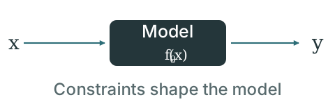
Use losses, constrained learning, or verification to shape the predictor.
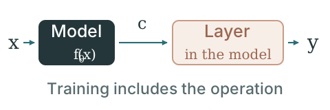
The task loss sees the output of a layer, completion, or solve.
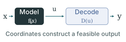
The model predicts coordinates for a feasible output map.
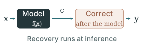
A downstream operation returns the decision used in deployment.
Try it: keep the candidate at (0.8, 0.8) and increase the penalty weight. Does the output reach the triangle at a finite weight? Then compare projection and feasible coordinates.
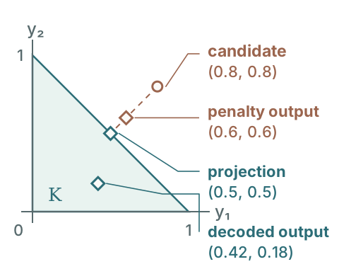
Notice that the quadratic penalty approaches the boundary, while projection reaches it. Switching projection between an output layer and post-processing keeps the same forward result; what changes is whether training accounts for it. Parameterization changes the input’s meaning: you choose coordinates that construct a feasible allocation.
Training-based approaches: change the predictor
Constraints can shape the training loss, the learning problem, or a verification-guided modification of the model.[2][3] The resulting predictor runs directly at inference. The important question is whether the method improves average behavior or establishes a property for every input in a specified region.
Structured layers: train through an output operation
A layer can transform a prediction, complete missing variables, or solve a constrained optimization problem. Training accounts for that operation, as in OptNet and differentiable convex optimization layers.[4][5] For our triangle, a projection layer returns the nearest feasible allocation and lets the predictor learn to anticipate the change. Feasibility comes from the forward operation and its numerical accuracy.
Constraint parameterization: predict feasible coordinates
Instead of predicting an allocation that may need repair, let the network choose two coordinates: is the fraction of the budget used, and is the share assigned to the first service. With both in , decode the allocation as . Its entries are nonnegative and sum to , so the budget rule is built into the output.
For example, and give . These coordinates describe how to construct a feasible allocation; they are not an allocation awaiting correction. The explorer lets you vary them directly.
Other methods use different feasible representations. ConstraintNet uses input-dependent vertex representations;[6] gauge-based approaches map a bounded reference region into the feasible set, with equality completion where required.[7] Check that the coordinates remain in their allowed domain and that the decoder returns feasible outputs. Also check coverage: a representation may omit useful feasible solutions.
Post-processing: recover the returned output
A correction or solver can turn a fitted model’s candidate into the decision that is actually used. Projection is one option; geometry-specific recovery and solver warm starts are others.[8] This can support stronger feasibility than the raw prediction, at the cost of extra computation and a possible change in output quality.
These roles can work together. DC3, for example, combines equality completion with differentiable inequality correction.[9] For the complete taxonomy and method-level details, see the prediction guide on GitHub.
From constrained prediction to constrained generation
In the allocation example, the model returns one decision for a given input. Now imagine planning a robot's route between two locations. Several routes may be useful: one passes to the left of an obstacle, another to the right, and others trade distance for clearance. A generative model offers a way to propose different candidates for the same task, learning the variation in possible solutions as well as their shared structure.
A generator uses random inputs to produce different candidates, optionally conditioned on context such as the robot's start and goal. Each returned route must satisfy the requirements for that context. We also care about the collection: its quality, diversity, and coverage, and how well it follows a target distribution when the task specifies one.
Generators construct candidates in different ways. Direct generators produce complete candidates; autoregressive generators build them through successive choices, which can be restricted by a grammar.[10] A diffusion sampler uses a learned denoiser or score to move through noise levels, with stochastic or deterministic updates. A flow-matching sampler integrates a learned velocity field from a prior toward a data distribution. We will focus on these iterative models, where constraints can enter during sampling as well as at the final output.
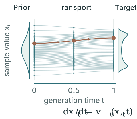
The prediction mechanisms still apply, but iterative generation adds a question about when they act. Should we guide an estimate of the finished sample, correct an intermediate state, or repair the final result? Each intervention can also change which feasible outputs are likely to appear. We therefore need to examine both where a constraint acts and how it affects the returned samples.
Constraints inside diffusion and flow sampling
Diffusion and flow models build a sample through repeated updates. For a robot planner, the sample is the whole route: a sampling step changes that candidate route, rather than moving the robot one step forward.
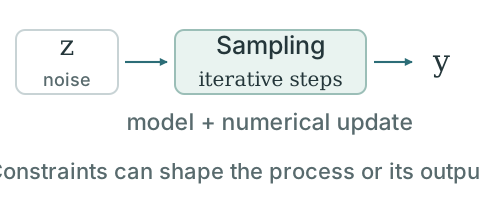
The key questions are what is constrained, and when. These four categories describe the intervention; each uses different information about the feasible set.
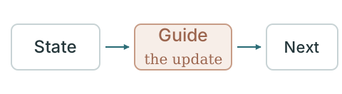
Steer sampling with an objective, often evaluated on an estimated final output. Better scores do not automatically mean exact feasibility.
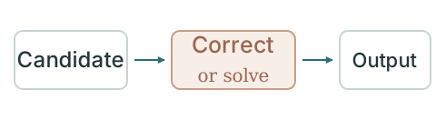
Apply a projection or solve to a state, an output estimate, or the final sample. The corrected quantity and timing matter.
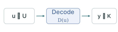
Generate coordinates in an allowed set and decode through a feasible map, as in our triangle example. The map determines which outputs are accessible.
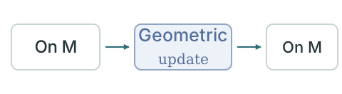
Build the dynamics around a domain or manifold . Feasibility relies on the modeled geometry and appropriate numerical updates.
Where do familiar methods fit? Universal Guidance illustrates objective-based steering.[12] Projected Diffusion and Physics-Constrained Flow Matching illustrate correction at different points in generation.[13][14] Riemannian Flow Matching and Reflected Diffusion use the geometry of the sample space.[15][11] Their algorithms differ; the categories identify the role that constraint handling plays.
Training supports these choices. A model can learn with constraint losses or with the decoder or correction that will be used at inference. Training changes model parameters; guidance changes the sampling computation. The complete classification, algorithms, and literature links are collected in the generation guide on GitHub.
Valid samples can still follow different distributions
For robot planning, clearing the obstacle still leaves a choice between useful routes. Constraint handling can change how often different routes appear. To see this distribution effect in a setting we can calculate exactly, return to the triangle. Draw proposals uniformly from and ask for uniform samples inside the triangle.
Compare the clouds: both methods return feasible points. Which one places more samples on the boundary, and does that match the uniform target?
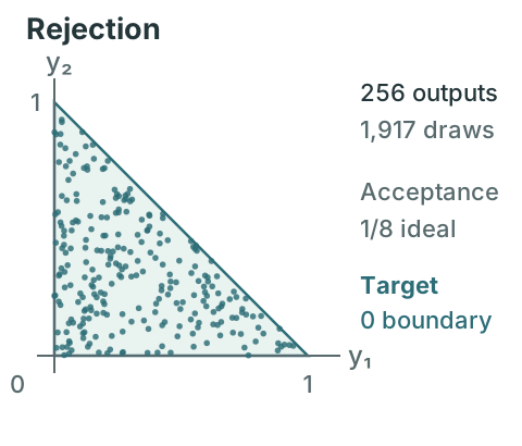
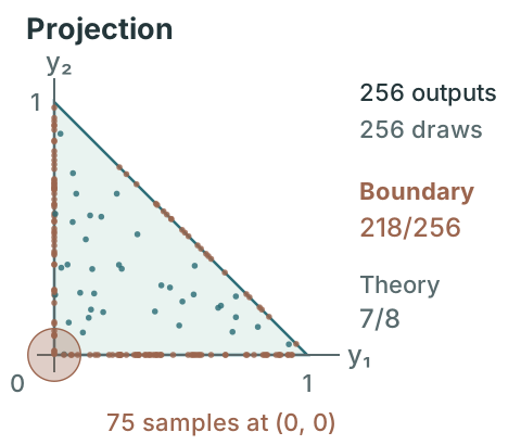
Rejection keeps feasible draws from the uniform square; independent draws and an exact membership test give the conditional target, with population acceptance . Projection returns feasible outputs from every proposal, but places population mass on the boundary, including at the origin. Both can be fully valid while following different laws. The same question applies after modifying diffusion or flow sampling: assess the complete output distribution against the task's desired quality, diversity, and coverage.
Choose from the operations you have
Start with the operations the problem makes available. The table gives useful starting points; the checks determine whether they fit your task.
| What you have | What to consider and check |
|---|---|
| A feasible representation or decoder | Consider parameterization. Check the coordinate domain, output coverage, and cost of constructing the representation. |
| A reliable projection, correction, or solver | Consider post-processing for an existing predictor or generator. Train through the operation when the model should anticipate its effect. Measure the entire procedure at the required tolerance. |
| A differentiable violation measure | Consider penalties or guidance to improve behavior. Establish final feasibility separately when the task requires it. |
| A cheap membership test | Consider rejection. Check the acceptance rate and whether the resulting conditional distribution is the one you want. |
| A test for valid sequence completions | Consider constrained decoding. Check that permitted choices still admit a valid completion. |
Include preparation costs: building a feasible representation may require vertex enumeration or a reference-point solve. A model used as a solver warm start should save time over a conventional initialization at the same stopping tolerance.
When the same constraints recur, extra training or preprocessing may pay for itself across many queries. When constraints change, online construction and enforcement costs matter more. Choose a pipeline whose assumptions fit the problem and whose output quality and complete cost meet the deployment goal.
Evaluate the result you will actually use
Four questions keep the comparison useful:
- Constraint satisfaction: What fraction of final outputs meet the chosen tolerances? Report equality and inequality residuals, including their largest values. State whether the evidence comes from a construction, solver, certificate, probability statement, or evaluated samples.
- Output quality: For prediction, report accuracy against reference outputs and the utility of the resulting decisions. For generation, examine quality, diversity, and coverage; assess fidelity to a target distribution when the task specifies one.
- Computational cost: Count preprocessing and training where relevant, then measure the entire inference procedure. Include checks, correction, decoding, failed attempts, and solver work. For generation, cost per valid sample can reveal what raw sampling speed hides.
- Applicable scope: Which constraint geometry, input region, oracle, solver condition, or discretization does the result require? A continuous-time property and a finite numerical implementation need a connecting argument.
Apply these questions to the returned object. If a model predicts an infeasible candidate and a solver repairs it, report the repaired decision's quality and the complete latency. If a relaxation is rounded, check the rounded output against the original rules. A feasibility-preserving component is useful only insofar as the later stages retain its property.
The triangle examples show why this view matters. A penalty can reduce a violation. A projection can make an allocation admissible. A coordinate map can build admissibility into prediction. Rejection and projection can produce valid populations with different probability laws. Each mechanism provides something valuable; the choice depends on what the application needs from the complete procedure.
For more methods and application-specific entry points, explore the Hard-Constrained Machine Learning repository. It follows our companion survey manuscript and links the literature on prediction, generation, applications, and evaluation. The manuscript's public preprint link will be added when available.
Selected references
- Fischer et al. DL2: Training and Querying Neural Networks with Logic. ICML, 2019.
- Chamon et al. Constrained Learning with Non-Convex Losses. IEEE Transactions on Information Theory, 2023.
- Zhao et al. Ensuring DNN Solution Feasibility for Optimization Problems with Linear Constraints. ICLR, 2023.
- Amos and Kolter. OptNet: Differentiable Optimization as a Layer in Neural Networks. ICML, 2017.
- Agrawal et al. Differentiable Convex Optimization Layers. NeurIPS, 2019.
- Brosowsky et al. Sample-Specific Output Constraints for Neural Networks. AAAI, 2021.
- Li, Kolouri, and Mohammadi. Learning to Solve Optimization Problems with Hard Linear Constraints. IEEE Access, 2023.
- Liang, Chen, and Low. Low Complexity Homeomorphic Projection to Ensure Neural-Network Solution Feasibility for Optimization over (Non-)Convex Set. ICML, 2023.
- Donti, Rolnick, and Kolter. DC3: A Learning Method for Optimization with Hard Constraints. ICLR, 2021.
- Geng et al. Grammar-Constrained Decoding for Structured NLP Tasks without Finetuning. EMNLP, 2023.
- Lou and Ermon. Reflected Diffusion Models. ICML, 2023.
- Bansal et al. Universal Guidance for Diffusion Models. CVPR Workshops, 2023.
- Christopher, Baek, and Fioretto. Constrained Synthesis with Projected Diffusion Models. NeurIPS, 2024.
- Utkarsh et al. Physics-Constrained Flow Matching: Sampling Generative Models with Hard Constraints. NeurIPS, 2025.
- Chen and Lipman. Flow Matching on General Geometries. ICLR, 2024.